Inventing Situations.

I’ve recently been doing some reading on machine learning with a mind towards applying some of my prior knowledge of representation theory.  The initial realization that representation theory might have some interesting applications in machine learning came from discussions with Chris Olah at the Toronto HackLab a couple months ago; you can get interesting new insights by exploring new spaces!  Over winter break I’ve been reading Bishop’s ‘Pattern Recognition and Machine Learning‘ (slowly), alongside faster reads like ‘Building Machine Learning Systems with Python.‘  As I’ve read, I’ve realized that there is plenty of room for introducing group theory into machine learning in interesting ways.  (Note: This is the first of a few posts on this topic.)

There’s a strong tradition of statisticians using group theory, perhaps most famously Persi Diaconis, who used representation theory of the symmetric group to find the mixing time for card shuffling.  His notes ‘Group Representations in Probability and Statistics‘ are an excellent place to pick up the background material with a strong eye towards applications.  Over the next few posts I’ll make a case for the use of representation theory in machine learning, emphasizing automatic factor selection and Bayesian methods.

First, an extremely brief overview of what machine learning is about, and an introduction to using a Bayesian approach to play RoShamBo, or rock paper scissors.  In the second post, I’ll motivate the viewpoint of representation by exploring the Fourier transform and how to use it to beat repetitive opponents.  Finally, in the third post I’ll look at how we can use representations to select factors for our Bayesian algorithm by examining likelihood functions as functions on a group.

Machine learning is essentially concerned with statistical modelling, with the main difference being that data is assumed to be cheap to gather and ubiquitous.  This is usually framed as a problem to be dealt with (“We need people who can deal with petabyte sized data sets!!!”), but also provides an opportunity to build more robust models and directly test the predictive power of the model.  With large data sets, one can use some data to build the model and hold back other data for testing the model, which helps to eliminate over-fitting problems.

Another feature of machine learning (especially if you read Bishop) is that there’s a strong focus on Bayesian approaches to probability.  I’ve taught Bayes theorem in calculus classes before, but hadn’t really come to understand the ‘Bayesian worldview’ until recently.  The Bayesian perspective is that probabilities are not the chance of a thing happening, but rather a measure of our certainty that the thing will happen, taking into account our existing data and (more controversially) our pre-existing assumptions and knowledge about the problem at hand.

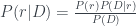
The Bayesian viewpoint is especially well-suited to learning environments.  Bayes’ theorem tells us that .  In English, consider as the event we’re interested in predicting, and as some data that we’ve observed.  Then the chance of happening given is determined by the overall probability of happening, the chance of the data appearing when is true, and scaled by the overall probability of the data occurring.

The part of Bayes’ theorem is the source of the historical controversy around Bayesian thinking: it’s called the ‘prior distribution,’ and asks us to start with an estimate of the overall probability of occurring, thereby bringing our assumptions and initial understanding of the problem into the calculation.  What happens in practice is that the prior distribution changes as we get more data, reflecting the better understanding that comes from further observation. Our initial assumptions matter less as we learn more about the world.  But let’s take a look at an example, to see this in action.

Rock-Paper-Scissors

Suppose we’re playing rock-paper-scissors.  In case you don’t know the game, it works like this: two players choose one of rock paper and scissors simultaneously.  Paper beats rock, scissors beats paper, and rock beats scissors.  It’s a simple game, usually used for breaking ties, but which has none-the-less led to an international organization and world championships.  (Henceforth, we’ll call the game RPS for short.)

Everyone knows the optimal strategy for a single game of RPS is to play uniformly randomly.  So instead, let’s play iterated rock-paper-scissors in a tournament setting, with known idiots.  In other words, pairs of opponents will play 1000 rounds of RPS, with the winner being whoever won more rounds.  And we’ll do this in a tournament, to see which players are the best overall.  Also, only one of the players in the tournament is uniformly random, and many of the players are idiots.

In this setting it’s no longer optimal to play randomly: if you can find patterns in your opponent’s play and exploit those patterns, you will rank higher overall in the tournament than someone playing uniformly at random (who will tend to end up in the middle of the pack).  In fact, there have been a few computer RPS competitions, like this one, where the best programs win about 80% of the time.  A good overview of basic strategies can be found here.

Humans are easy to beat, it turns out: here’s a robot with a 100% win ratio using really fast recognition of the opponent’s hand, and here’s an applet from the New York Times that wins a bit more honestly.  By the way, Shawn Bayern (a computer scientist turned law professor) has generously lent me the dataset used for making the NYT applet for teaching and my own experiments.

If you have two ‘smart’ players playing against one another, you get some very interesting interactions.  You win by finding patterns in the opponent’s moves while attempting to appear random yourself.  Even though RPS is itself kind of a silly example, the techniques we’ll see have broad potential for application. The problem of finding patterns in a stream of characters which the source of the characters is actively trying to conceal should be quite applicable to cryptanalysis.  And the general problem of finding patterns in streams of character data has obvious applications to biology (think GATTACA).

Bayes’ Theorem as Algorithm

So our problem is a problem of pattern recognition:  How can we use Bayes’ theorem to detect and exploit patterns in an opponent’s play?

The Bayes-bot I’ve built does it in the following (pretty standard) way.  First, set a memory parameter M, which will tell the bot how many of our opponent’s moves to keep track of.  Then, for each of the possible strings of M moves, we will keep track of how many times we’ve seen the opponent play rock paper, or scissors (a vector of three natural numbers).  We initialize each of these vectors at , which effectively sets our prior distribution to assume that the opponent plays uniformly at random.

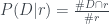
As we play, we update the tables after each observed move, and use the tables of past data to figure out what to do next.  We look at the M immediately previous moves of the opponent; this is our data, .  We can now estimate the probability that the opponent chooses (say) rock:
.

We estimate as the number of times we’ve observed over the total number of rounds so far, N.  Write this as .  Likewise, is the number of times we’ve observed our data immediately followed by previously: it’s the entry in our table, divided by the total number of times we’ve observed r.  Then .  Finally, we estimate the probability of the data occurring by .

Putting this all together in Bayes’ theorem, our formula simplifies to the very concise:
.

We can calculate probabilities for paper and scissors similarly.  If we take a frequentist approach, we then just choose the most likely of the three options, and play a move to beat it.  Alternately, we can use a random variable to choose one of R,P,S using the distribution we’ve just generated.  The latter approach works much better: if the probabilities are sharply ‘peaked’, then we’re more sure of what the opponent is going to do.  If there’s less of a peak, then we’re less sure.  Correspondingly, if one probability is slightly more than a third and the others are slightly less, it doesn’t make sense to always pick the slightly-more-than-a-third option; we’re just not that sure, and our data might be slightly skewed, anyway.  And if we always pick the most likely option, we may introduce unintentional patterns in the way we’re playing which can be exploited by a smart opponent (see also: use randomization in mixed strategies).  We’ll call the ‘always-pick-the-biggest’ strategy the Frequentist, and the ‘pick-according-to-the-distribution’ strategy the Bayesian.

There are problems, though!  First, our ability to find big patterns is limited by our choice of M.  And furthermore, the number of observations we need in order to make confident predictions of non-randomness is exponential in M.  It turns out that when playing a 1000 rounds of RPS, this algorithm does best at M=3 or 4, and then falls off dramatically.  The Frequentist M=3 and M=4 bots tend to do about equally well, and come out ahead of the M=5 and M=6 bots.  These bots don’t have enough data to move strongly away from the starting uniform distribution in 1000 rounds of play, and tend to land closer to the middle of the rankings in the tournament.

Each of the prior moves we track (along with how many moves ago they happened) is a ‘factor’ in building our model.  The more factors we track, the more data we need in order for our model to converge.  A fantastic learning algorithm, then, will be able to identify a pattern quickly in order to exploit it.  And our analysis suggests that if we can find a few really good factors then we’ll do better than looking at lots of irrelevant factors, while also reducing the time to convergence.

The question, then, is how can we automatically find significant factors for building a model of how our opponent acts?  The significant factors for one opponent won’t necessarily match those of another, after all.  If we play against Edward Scissorhands, the most significant factor is that his hands are scissors.  On the other hand, if we play against someone who plays to beat my previous move every time, the most significant factor is my last move.

This is where representation theory kicks in.  We can think of our moves as elements of the cyclic group, and then use representations to find better ways to pick our data.  I’ll expand more on how to do that that in the next couple posts.