Inventing Situations.

Suppose you’re building a widget that performs some simple action, which ends in either success or failure.  You decide it needs to succeed 75% of the time before you’re willing to release it.  You run ten tests, and see that it succeeds exactly 8 times.  So you ask yourself, is that really good enough?  Do you believe the test results?  If you ran the test one more time, and it failed, you would have only an 72.7% success rate, after all.

So when do you have enough data, and how do you make the decision that your success rate is ‘good enough?’  In this post, we’ll look at how the Beta distribution helps us answer this question.  First, we’ll get some intuition for the Beta distribution, and then discuss why it’s the right distribution for the problem.

The Basic Problem

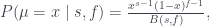
Consider the widget’s tests as independent boolean variables, governed by some hidden parameter μ, so that the test succeeds with probability μ.  Our job, then, is to estimate this parameter: We want a model for P(μ=x | s, f ), the probability distribution of μ, conditioned on our observations of success and failure.  This is a continuous probability distribution, with μ a number between zero and one.  (This general setup, by the by, is called ‘parameter estimation‘ in the stats literature, as we’re trying to estimate the parameters of a well-known distribution.)

The ‘natural’ distribution to consider for P is the Beta distribution.  This is given by:

where is the Beta function, which normalizes the P so that its integral is 1. (As it turns out, , when s and f are integers.)  I’ll come back to why the beta distribution is a ‘natural’ choice later.

Looking at this formula and the plot of P for eight successes and two failures, a few things stand out.

• The formula is going to have asymptotes if s or f are zero.  It’s generally a good idea to include ‘phantom’ observations of one success and one failure.  We’ll do this in all of the plots to come.  (More on this later, in the discussion of why the Beta distribution is natural.)
• The numerator indicates that P is 0 at x=0 and x=1 whenever s and f are bigger than 1, which provides a small sanity check: Once we observe a failure, it’s impossible for μ to be 1.
• The peak of the distribution is actually different from the mean.  If you’ve only ever looked at normal distributions, this is may be surprising: the beta distribution has a more complicated shape than a normal distribution.  In this case, the most likely value of μ based on our observations so far is bigger than 0.8.  (In fact, it’s about 0.87.)
• The expected value of the probability distribution is 0.8, exactly the ratio of successes.
• Once we add a phantom success and failure, the most likely value (MLE) becomes 0.8, the ratio of observed successes, but the expected value is a bit lower. In fact, this is always the case: With the phantom success and failure, the MLE is .
• The cumulative distribution function (CDF) is P(μ>x).  This is super useful for picking a confidence bound, and answering questions like ‘what’s the value x where we’re 90% sure that μ is greater than x?’  (In this case, that bound is just 0.633.)

So just going with the maximum likelihood estimate isn’t giving us very much certainty about μ, precisely (as it turns out) because we haven’t collected enough data yet.  What happens when we collect more data?  Here’s four plots with more observations and the same overall observed success ratio, with a phantom success and failure thrown in.

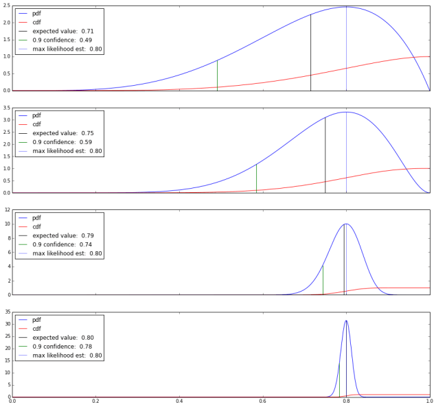
As we add more data, the PDF becomes more and more tightly distributed around the expected value, 0.8: We have more certainty that the expected value is really close to the observed success ratio.

What we’ve gained by looking at the distribution is a concrete way to measure our certainty about our estimate of μ. This is kinda great.  By the time we’ve collected a thousand observations here, we’re pretty sure that μ is at least 0.79.

We also open ourselves up to a new testing strategy: By setting a confidence cutoff, we can run tests until we’re reasonably sure that we’ve passed the bound, and then stop.  In this example, we can stop a little while after the hundredth test, when we’re 90% certain that μ is at least 0.75, which was the launch criteria.  If the distribution tells us we’re doing great, we can stop earlier and save time on testing.  (Conversely, we can set an upper bound, so we can stop testing when we’re pretty sure we’ve missed the target and tell the engineers to go back to the drawing board.)

Why is the Beta Distribution Natural?

This comes down to Bayes theorem and some nice properties of the Beta distribution. Applying Bayes theorem to P(x=μ | s, f), we get:

The right side breaks up into three parts: The likelihood function, P(s, f | μ=x), is easy to compute: It’s .  The denominator is a normalizer, which ensures that the total probability is one.  Which leaves just the prior distribution, P(μ=x) to worry about.

It turns out that the Beta distribution is self-conjugate, meaning that when the prior P(μ=x) is a beta distribution, then P(x=μ | s, f) is a Beta distribution as well. It also turns out that P(x=μ | 1, 1) is the uniform distribution on [0, 1].  So, if we start the day with the belief that μ is equally likely to be any number in the range [0, 1], then we end up with a Beta distribution P(x=μ | s+1, f+1) as the posterior.

And this is why the Beta distribution is natural to consider, and why it makes sense to add a ‘phantom’ success and failure.  (Some people prefer to add a half a success and half a failure.  This is called the Jeffrey’s prior.  It gives less weight to the phantom observations, and – due to the non-uniform shape of the distribution – slightly favors the hypotheses that μ is either large or small. But I like integers and the uniform prior, personally.)

Endnotes

The approach we’ve take here is pretty Bayesian.  In addition to using Bayes theorem once, we’re also working directly with the distribution here, and taking the stance that our computers can handle the computations and arrive at numerical answers.  As opposed to imposing assumptions that the distribution is roughly Gaussian for the sake of generating big plug-and-play formulae.  (Incidentally, the methods presented here are essentially a one-sided version of the Jeffrey’s Interval.) We’ve also made no null hypotheses nor computed associated p-values to get where we wanted to go: Our basic assumption is that our tests are independent, and that μ could equally well be any number prior to making any observations.

The beta distribution can be found in the scipy.stats package in Python.  The plots in this post were made with matplotlib.