Recently I’ve been playing with building a regression model for the brightness of images produced with the Raspberry Pi’s camera board. Essentially, I want to quickly figure out – hopefully from a single image – what shutter speed and ISO to choose to get an image of a given brightness.
This is a pretty standard regression problem: We some data, extract some information from it, and use that information to make a prediction. To get a better handle on the algorithms involved, I wrote my own code to perform the regression, using NumPy for fast linear algebra operations. You always learn something from re-inventing the wheel, after all.

Gathering Data
With the Pi camera board and recent firmware, we can choose shutter speed (to a maximum of 2.5 seconds) and ISO. Shutter speed controls how long the sensor collects data for: long shutter speed can cause motion blur if you have fast moving subjects. ISO controls sensitivity of the sensor, and can be set between 100 and 800, with higher numbers meaning more sensitivity in the sensor. Higher ISO leads to a brighter image, but with more noise in the image produced. The combination of SS and ISO determines the overall brightness of the image.
To take a picture in Python, I’ve been using a system call to the `raspistill` command. (Recently, there’s been work on building a pure Python library for the camera to eliminate the need for system calls, but I haven’t switched over yet. See here.)
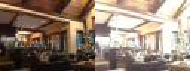
For data collection, I’ve built up a small library of pairs of images (about 500 pairs of images, as of this writing). These images are not big: 64×48 pixels. But they are large enough to give me some data to play with, and small enough that I can extract information pretty quickly. The initial picture (the ‘base’ image) is always taken at 100 ISO (to minimize noise) and a fixed shutter speed of 3/4 seconds. This provides a reference image from which we can extract useful information. For the purposes of building the regression, I also take a second image of the same size at a random SS and ISO, which I call the ‘test’ image.
For each pair of images, we convert both to greyscale (with 256 possible pixel values) and extract the following information:
- Base brightness: The average brightness of the base image, obtained very naively, just as the median of the pixel values in the image.
- Base Variance: The variance of the pixels of the base image. This should tell us roughly how evenly distributed the different pixel values are.
- Base Lower Cutoff and Upper Cutoff: These two numbers tell us two lower and upper bounds between which lie 90% of the pixels in the base image. (These turned out to be very useful data factors, and halved the error in my regression when I began including them.)
- Test brightness: Average brightness of the test image.
- Test SS: Shutter speed of the test image.
- Test ISO: ISO of the test image.
There are other choices of factor that I haven’t included (yet), which should improve the quality of the regression model, including using the full greyscale histogram from the base image. This would give 256 additional factors; as soon as we move to a quadratic model, we’ll then have more factors than data, which is a problem for simple regression. So to deal with more factors, I’ll need to implement some automatic feature selection…. A future post, hopefully.
When we take a picture in the field, we’ll then specify two out of the three ‘test’ properties (brightness, SS and ISO). The camera will then take a ‘base’ picture, and use the properties of the base image and our specified test properties to try to produce the third test property. For example, choosing brightness and shutter speed is analogous to using ‘shutter priority’ with a standard digital camera: the regression model tries to guess a good ISO to produce the desired brightness with your supplied shutter speed. On the other hand, specifying SS and ISO asks the model to guess what brightness we can expect from an image taken with those parameters.
The Regressor
Because I was interested in implementation details, I wrote my own regression algorithm instead of using a pre-packaged library. For matrices and such, I’m using NumPy (which gives me very fast linear algebra routines). I’ve been writing my regression in Sage so I can take advantage of some simple polynomial operations. Finally, I’ve been using the Python Imaging Library (PIL) for all of my basic image manipulation needs.
The regression is performed by a pretty general ‘regressor’ class that I’ve developed. To initialize the regressor, we tell it what kinds of data factors to expect (key names, expected mean value for the data factor, and a scaling constant), and what degree D of polynomial fitting we would like. It then treats each input factor as a variable, and builds a general degree D from these variables.
The regressor is then fed data in the form of small dictionaries, which must have keys corresponding to each of the expected data factors. The regressor then builds a vector of polynomial data from this input. These vectors can be considered as forming a (probably very large) matrix 


Initially, I was just building a giant matrix
Notice that the matrix 


When we’ve passed all the data we’re interested in through the regressor, we can then ask it for the best-fit function.
An interesting implementation detail: While it’s not super useful for this project, I noticed that this gives us an interesting opportunity for dealing with situations where we want a ‘constantly learning’ regressor. Since the footprint of the regressor never grows, we can leave the regressor ‘on’ and just update them with new data as it becomes available, and solve for a best fit function on request. In fact, this is how the regressor class is implemented.
But we can also introduce a variable 


Good Data Hygiene
To get a somewhat rigorous model, we need to divide our data into training data and testing data.
I’ve used a folding process, arranging my 500 pairs of pictures into five or ten folds, and then building one regressor for each fold. The regressor uses its associated fold only for testing, and uses all of the other folds for training. Thus, with 500 pictures and five folds, each regressor will have a training set of 400 images and a testing set of 100 images. With ten folds, each regressor is trained on 450 images and tested on the remaining 50 images; we get a larger training set but a bit less certainty about its error on testing.
Some Results
We have three possible target variables, brightness, shutter speed, and ISO, so I’ll give results for each separately.
- Brightness: This has usually been my go-to testing case: Can I guess the brightness of the image at a given shutter speed and ISO? A straight linear regression (degree 1) gives an average error of 22 points out of 256, or 8.5% of the possible range of values. Using a degree two regression, we achieve an error of 10.8 points, or 4.2%, which is a marked improvement. At degree 3, we get about the same error on average, but the errors produced by each regressor are more erratic. In the degree three case, there are 84 factors (six input factors combined in all possible ways to achieve a monomial of degree 3 or less) which suggests that this is the threshold where over-fitting becomes a problem. Clearly I need to be using some more robust feature selection…
- Shutter Speed: This is the feature I’m most interested in getting a good regression for, since I usually want my ISO to be 100, for minimal noise. Unfortunately, it’s also where the regression is having the least success so far. The linear regression gives an average error of about 1/3 of a second, which is fairly significant, but possibly still usable. The quadratic model and cubic models are only marginally better, again with more erratic behaviour in the cubic case.I did a bit of additional analysis of the outcomes of the shutter speed regression: I’m mainly interested in having a target brightness of 100, so it makes sense to ask about error when the brightness is near 100. In this case, the error seems to drop to about 1/4 second, which is significantly better.
- ISO: The results for ISO are somewhere between the SS and brightness results. The linear model gives an average error of 119 points out of a possible 700, while the quadratic model improves to an average error of 81 points.
The results aren’t very pretty, all told, but are potentially usable. I’ve written some other code which tries to adaptively find the right SS/ISO combination adaptively, by scaling the SS relative to how far off we are from the target brightness. Currently, this adaptive process takes about 8 or 10 seconds in normal conditions, but the regression should provide a better initial guess, brining down the calibration time when I start a new timelapse.
Going Forward
It looks like the regression for shutter speed is producing something vaguely usable; potentially, it could do better with significantly more data to work with, since we would then be able to fit higher degree polynomials with more confidence. Meanwhile, given the variation in possible conditions for taking a picture, it isn’t clear what the best possible outcome would look like. I’m also interested in figuring out how to do some automatic feature selection, which should allow me to fit higher degree polynomials with the same amount of data.
I also need to write some code so that the regressor can output some basic python code that I can drop into my Raspberry Pi, which (in spite of my prior work on the matter) isn’t running Sage, mainly because I want to keep resources free for the timelapse program. Once this is done, we could get some real field tests of the regression!
