Roshambo Part II – Fourier Analysis

In the last post, we looked at using an algorithm suggested by Bayes’ Theorem to learn patterns in an opponent’s play and exploit them. The game we’re playing is iterated rock-paper-scissors, with 1000 rounds of play per game. The opponent’s moves are a string of choices, ‘r’, ‘p’, or ‘s’, and if we can predict what they will play, we’ll be able to beat them. In trying to discover patterns automatically we’ll gain some general knowledge about detecting patterns in streams of characters, which has interesting applications ranging from biology (imagine ‘GATC’ instead of ‘rps’) to cryptography.

Fourier analysis is helpful in a wide variety of domains, ranging from music to image encoding. A great example suggested by ‘Building Machine Learning Algorithms with Python‘ is classifying pieces of music by genre. If we’re given a wave-form of a piece of music, automatically detecting its genre is difficult. But applying the Fourier transform breaks the music up into its component frequencies, which turn out to be quite useful in determining whether a song is (say) classical or metal.

This goat recognizes and apparently enjoys metal. Possibly using a furrier transform... — This goat recognizes and apparently enjoys metal. Possibly using a furrier transform… (sorry.)

The waveform for a music sample is simply an association of an intensity of the signal with each moment in time. At time t, we have an intensity $f(t)$ . Thus, our waveform is really a function of time. But Fourier analysis is concerned with periodic functions, which repeat themselves exactly after a given amount of time. Thus, it’s useful and standard in Fourier analysis to assume that time is cyclic: Our piece of music starts over again as soon as it is finished. If you look at very short samples of music, you see that this is fairly reasonable: from one millisecond to the next, the waveforms in music usually look quite similar.

A short sample from a song I made last summer. The overall waveform changes, but locally is fairly periodic.

When working with computers, our storage of the waveform is necessarily discrete: it will consist of many samples of the intensity of the signal, instead of a continuous representation of the signal. Let’s suppose our music consists of 256 samples (which is very small for a piece of music). Note that everything that follows works fine for an arbitrary number of samples, not just 256.

And now I should tell you about the cyclic group, $C_{256}$ . We can also (with some knowledge of Euler’s Identity) think of the group $C_{256}$ as the set of numbers of the form $e^{i \pi x}$ , with $x$ any fraction with denominator 256. This gives 256 points evenly distributed around the unit circle in the complex plane. Multiplying any two of these numbers together gives another such number, and they ‘wrap around’ the circle in exactly the right way.

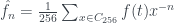
Our samples are then a function $f$ which assigns an intensity to each of the elements of $C_{256}$ . The function will have 256 Fourier coefficients corresponding to 256 different possible frequencies in the data. The n-th Fourier coefficient can be written down with the following formula:

$\hat{f}_n = \frac{1}{256}\sum_{x\in C_{256}} f(t)x^{-n}$ .

There are a couple important facts to note here. Firstly, the Fourier transform completely determines the function: If I know all of the Fourier coefficients, I can reconstruct the original function exactly. This is done using the inverse Fourier transform:

$f(t) = \frac{1}{256} \sum_{x\in C_{256}} \hat{f}_n x^n$

Secondly, thinking carefully about the zero-th Fourier coefficient, we might notice that it encodes the mean value of the entire set of samples: When we perform the forward transform, we take the sum of all of the samples. If we throw away all but the 0th component, and then take an inverse transform, we’ll just be dividing this sum by 256, giving us the mean value. The 0th component encodes where we are on average, and the other components encode precisely how we vary around that mean.

Back to RPS

How can we use the Fourier transform in our problem of finding patterns in games of RPS?

First, we convert our string of moves into a list of numbers, -1, 0, and +1 for rock, paper, and scissors respectively.

We can now think of each of this list as a signal, and apply the Fourier transform to try to look for periodicity in the signal. Taking the Fourier transform now gives us a list of signal intensities at different frequencies; if there is periodicity in our signal, then some of our frequencies will have strong signals. Great!

Unfortunately, the information may not be immediately useful for figuring out what the actual periodicities are! This is because the Fourier transform assumes that the whole signal is periodic. Suppose we work with a signal whose period is nine, but we have a total string that is 1000 characters long. Then we see lots of length-nine repetition visually, but when we wrap back around at the end of the string, we’ve introduced an off-by-one skip. This will still show up as some kind of strong frequency in our Fourier series, but not at the 9th frequency, as we would hope. Additionally, this method of looking for periodicity may not be very robust to noise in the signal, for example if our opponent plays with some randomness.

In my own testing of this procedure on a sequence of period nine and length 1000, I tended to see strong signal at frequencies that were multiples of 111. Taking shorter samples gave more reasonable answers, though; there’s certainly merit to the approach.

But let’s change perspective a bit…

Probably a Better Approach

Let’s apply a more probabilistic approach to looking for periodicity. If we have a truly periodic opponent, operating with period k, then their behaviour is dependent entirely on what they did k moves ago. Then we could look through the move history and see if it’s consistently the case that each move is the same as the move n plays later, for each possible value of n. We would see good consistency for k and be able to identify that as the period of the opponent’s play.

But what if our opponent instead looked k moves back, and then flipped a coin: With 50% chance they play the same thing they did k moves ago, and with 50% chance they choose a different move at random. They will still play the same thing 50% of the time, which is more than the 22% of the time that we would expect of a totally random player. It would be great if we could still identify the periodicity here, even though there’s a fair amount of noise.

Then we should try to estimate the probability of (say) rock, given that their play k moves ago was rock. This is exactly a conditional probability: $P(r|D)$ , where D stands for ‘k moves ago the opponent played rock’. If our move list is a sequence $m=(m_1, m_2, \ldots, m_N)$ , then we could rewrite the probability as: $P(m_N=r|m_{N-k}=r)$ .

To compute this conditional probability we can use Bayes’ theorem, just as we did last time.

$P(m_N=r|m_{N-k}=r)=\frac{P(r)P(m_{N-k}=r|m_{N}=r)}{P(m_N=r)}$ .

We can even re-tool the algorithm we developed last time to figure out a good estimate of this probability.

Consider the conditional probability on the left side of Bayes’ theorem, $latex P(D|H}$. This is called the likelihood function. If we keep the hypothesis H fixed and allow D to vary across all possible (disjoint) values, the likelihood function gives probability distribution on the possible data, given that the hypothesis is true. In particular, 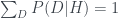$\sum_D P(D|H) = 1$ .

Now, if I make an imaginative leap, I could think of the data as being points in $C_3$ : I’ll just associate each of the values r, p, and s with one of the numbers in $C_3$ . This isn’t a huge leap, it turns out: our set of possible data has a number of symmetries, and $C_3$ encodes those symmetries. Now our probability distribution is a function on $C_3$ , and we can take its Fourier transform…

Fourier Transforms of Probabilities

First, let’s consider the uniform distribution U, where r, p, and s are equally likely. Then $P(r|r)=P(s|r)=P(p|r)=\frac{1}{3}$ . The Fourier transform of this distribution is $\hat{U}_0=1$ , and $\hat{U}_1=\hat{U}_2=0$ .

Since the 0th Fourier coefficient is always just the sum of the function values, then the 0th frequency is always 1 regardless of what our probability function is. The uniform distribution just happens to have 0’s in the other ‘frequencies.’ Any non-uniformity in the probability function will appear as non-zero coefficients in the first or second frequency.

As a result, taking the Fourier transform of the likelihood function gives us a great way to measure how non-uniform our probability distribution is. Thus, if we see ‘big’ non-zero Fourier coefficients outside of the trivial component, we have a non-random distribution.

But the situation is actually even better than we were looking for. Non-uniform distributions will arise both in cases where the output is periodic and when the output is ‘anti-periodic.’ This happens, for example, if you decide to play anything except the move you used k moves ago.

For example, if the opponent is anti-periodic and played rock k moves ago, they will play either paper or scissors this turn. Then if you play scissors you are sure to either tie or win. This, by the way, leads to some concreate advice for beating your friends and getting your way in critical games: People tend not to repeat themselves as often as they should, so a reasonable strategy against humans is to play the thing that their last move would have beaten. (Or at least until they start to catch on.)

But in any case, if the sequence of moves is non-uniform, our probabilistic approach will detect the non-uniformity and tell you directly how to exploit it.

Representations

In fact, the Fourier transform is exactly a process of breaking up a function on the cyclic group across what are called irreducible representations. The utility of the Fourier transform comes from the fact that the frequency spaces are orthogonal: In other words, there exists an alternative metric which takes into account the cyclic nature of the cyclic group, and the Fourier transform breaks up functions into components which respect this special metric. The Fourier transform is helpful exactly when there are interesting periodicities in our space of possible data.

More generally, mathematical groups are measures of symmetry in a system. Instead of having ‘frequency spaces,’ a general group has irreducible representations, and breaking up a function across the irreducible representations is exactly analogous to the Fourier transform. If our space of possible data has group-like structure on it, we can use representation theory to break our function into orthogonal parts with respect to a metric that takes symmetry into account. Just as with the Fourier transform, we should then be able to see quite clearly whether our probability distribution is uniform or not.

In the next post, I’ll expand further on these ideas, and show how to extend our algorithm to considering more than one prior move at a time. And I’ll also think about a variant game where you have to choose three roshambo moves at a time.

Inventing Situations.

tom denton on math and things.