 This week I was surprised to learn that I won the Kaggle Social Networks competition!
This was a bit different from other Kaggle competitions. Typically, a Kaggle competition will provide a large set of data and want to optimize some particular number (say, turning anonymized personal data into a prediction of yearly medical costs). The dataset here intrigued me because it’s about learning from and reconstructing graphs, which is a very different kind of problem. In this post, I’ll discuss my approach and insights on the problem.
Competition Background
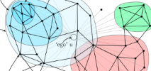
Kaggle is a data science competition site; given a ‘large’ dataset, participants try to find algorithms which extract useful data to optimize against some ground truth. For this particular competition, the data consisted of social circles from Facebook, and accompanying anonymized data. For example, you would have the list of John Doe’s friends, along with all of the ‘friend’ relationships amongst his friends, where people have lived and worked, where they went to school, what languages they speak, and so on. All of the names of people and places are replaced with sequential numbers to prevent reconstructing identities from the data.
Each John Doe would then indicate their social circles within their set of Facebook friends. These social circles might overlap (for example, if you had a ‘work’ circle and a ‘family’ circle, and happened to work at a family business) or not. It also wasn’t necessary that every friend appear in at least one circle. So the circles were quite free-form. Given the Facebook data, the task is to reconstruct the set of social circles.
The Kaggle data is divided into three sets: Test, Public, and Private. The test data is data with solutions that you’re given as ground truth for designing and fine-tuning your algorithms. The Public and Private sets are just data without solutions. As you make submissions throughout the competition, your solutions are scored against the Public dataset and put on a leaderboard. The results at the end of the competition, though, are determined by the Private dataset, where your solutions are scored at the end of the competition.
I worked for probably a week or week and a half on the problem; I believe I peaked at 7th place on public leaderboard. I stopped working on the problem when I moved at the end of August. By the end of the competition in late October, I was ranked 67th on the Public leaderboard.
It’s well-known that people tend to over-fit the data in the Public leaderboard. In this case, there were a total of 110 data instances, of which ‘solutions’ were provided for 60. One third of the remaining 50 instances were used for the Public scoring, and two-thirds were used for the Private scoring. I got the sense from my work with the Test data that the Public set was a little bit strange, and so I tried to restrain myself from putting too much work into doing well on the Public leaderboard, and instead on understanding and doing well with the Test data. This seems to have worked well for me in the end.
Some Notes on the Data
Examining the test data, it was clear that there was a great deal of variation in how people identified their social circles, as well as variation in the size and density of their friend networks. For example, some people very carefully placed every one of their friends into some circle, with all circles completely disjoint, while others had just a few large circles with significant (over 80%) overlap. This meant that the overall dataset was actually pretty small relative to the degree of variation.
Second, there’s a great deal of variation in the Facebook demographic data. Amongst my actual Facebook friends, some people flesh out their whole profiles with every school they’ve attended since they were six years old, and other leave everything blank that they can get away with and use a fake name besides. Most people fall somewhere in between, and often don’t update their current location or job if their status changes. This suggests that the Facebook demographic data can be pretty unreliable.
I made some initial attempts at using the demographic data, but eventually completely abandoned it, sticking to using just the graph data. My rationale was that the demographic data should be replicated in the graph data for people with meaningful connections, which saves me from trying to infer who left something blank or didn’t update their profile. Additionally, knowing that a set of friends attended the same university might be sufficient to generate a circle, but that circle could easily be far too large if someone had a few different, non-overlapping interests while they were in school; the equestrian team and the bee-keeping society might have a small intersection. The graph data itself should have the ‘right’ level of granularity built in, in a way that pre-selected demographic data cannot.
Third, the actual evaluation metric used in the competition has a real effect on the optimal strategy for constructing circles. The metric was the ‘edit distance’ between our predicted circles and the ground truth. After an initial best matching of our predicted circles and the ground truth, we count the number of edits required to turn the prediction into the ground truth. An edit consists of adding a person to a circle, deleting a person from a circle, creating a new empty circle, or deleting an empty circle.
Given the volatility in how the ground truth circles were labelled, I decided to focus on identifying a few large circles that were almost certainly correct. Luckily, large circles have the biggest impact on the final score, and are also easier to detect.
Algorithms
My final solutions used the following process:
- Compute an approximation of the exponential adjacency matrix
of the friend graph. The adjacency matrix
of the friend graph is simply the matrix of connections. The exponential adjacency matrix is the sum of
. The nth power of the adjacency matrix counts the number of length-n paths between various vertices; taking the exponential is summing up paths of all lengths, weighted by length of the path. Conceptually, it gives a better notion of the degree of connectedness of various nodes, by smoothing out inconsistencies in the basic adjacency matrix. For example, if vertices A and B have many common neighbors but no edge directly connecting them, then the AB-entry of the adjacency matrix is 0, but the entry in the exponential adjacency matrix will be quite high. This helps to fill in connections between people who ‘should’ be friends.
- Apply a generic clustering algorithm using the rows of the
Spectral clustering works by computing a similarity matrix for the data, and then using some of the eigenvectors of that similarity matrix to reduce the dimensionality of the data. Clustering is then performed on the lower-dimension reduction. I think that the use of the exponential adjacency matrix helped quite a bit here, since it naturally accentuates the similarities in the adjacency matrix. It might be worth following up the particular interaction between the exponential adjacency matrix and spectral clustering algorithms. I found that setting K=10 for people with more than 350 friends and K=6 for fewer than 350 friends worked well for the test data.
- Throw away low-density circles. For a circle with
people, define the density as the number of edges in the circle divided by
(the maximal possible number of edges). Any circle with density less than 0.25 was thrown out. (This threshold was arrived at by grid search, and then bumped up a bit to be conservative.)
- Augment the remaining circles by adding in people with more than F friends in the circle, or if they are friends with at least 50% of the people in the circle. For graphs with more than 250 vertices, we set F to 8, and otherwise set F=6.
- Include small connected components with at least 5 members and no more than 15 as independent circles.
- Merge circles with more than 75% overlap.
There are clearly a number of arbitrarily chosen constants here. The overall size of the dataset was far too small to try to ‘learn’ the right values of these constants. I tried at one point bucketing the dataset into four or five classes of circle by circle size, and learning the right constants, but ended up with wildly over-fitted results. In the end, it was down to choosing ‘reasonable’ constants and hoping for the best.
Conclusions and Reflections
It was really fun to work on a graph learning problem! Many thanks are due to Julian McAuley for organizing the contest.
Honestly, I was pretty excited to try out using graph Fourier transforms as feature vectors, but didn’t end up doing this because the Fourier transforms are too slow once we have a graph with more than about 400 vertices… Alas. I still think it would be an interesting approach for smaller circles, though!
The main take-away for me from this contest is that personal data (like university, workplace, and so on) ended up mattering less than the actual structure of the graph. The personal data might be too fine or too coarse to actually capture the social relationships of an individual, but the web of actual connections encodes that structure directly. Another interesting follow-up question is how to ask for data that’s actually more useful in recovering community structure. It might be more useful to have people provide self-defined ‘tags’ describing their interests or communities.
There’s a game called ‘advanced chess’ in which human players use chess computers to explore possible moves, and then move as they will; the exploration here felt similar. I had a number of heuristic ideas which I would code up and watch the outcome of, and then discard the ones which didn’t perform as well. In the absence of a proliferation of training data, one is forced into heuristic choices by necessity. My final solution was a nice mathematical idea (use spectral clustering on the exponential adjacency matrix) augmented by a handful of simple heuristics.
And ultimately, this isn’t an unusual occurrence. The funny bit about Kaggle competitions is that you’re learning with labelled data. Outside of Kaggle, you often don’t actually have training labels, and a major part of the learning problem is figuring out what data to collect in the first place. The size of the data set here almost certainly reflects the difficulty of getting ground-truth data on social circles.
