Principal Component Analysis via Similarity

Recently I’ve seen a couple nice ‘visual’ explanations of principal component analysis (PCA). The basic idea of PCA is to choose a set of coordinates for describing your data where the coordinate axes point in the directions of maximum variance, dropping coordinates where there isn’t as much variance. So if your data is arranged in a roughly oval shape, the first principal component will lie along the oval’s long axis.

My goal with this post is to look a bit at the derivation of PCA, with an eye towards building intuition for what the mathematics is doing.

Suppose we have a matrix of data X, whose rows $X_1, \ldots, X_n$ are data points, and whose columns are the feature values of the data points. To be overly concrete, suppose we have a matrix recording whether each of six people has watched each of four movies. Thus, we have a 6×4 binary matrix.

Our first job is to clean up the data a bit by removing the column means from each of the data points, so that all of the features have mean zero. We’ll call this adjusted matrix $X_m$ .

Once we’ve ‘demeaned’ the data, we compute two very important related matrices, the scatter matrix and the Gram matrix. PCA is fundamentally a way to extract important information from the scatter matrix. The scatter matrix is $S:=X_m^tX_m$ , and the Gram matrix is $G:=X_mX_m^t$ . The entries of the scatter matrix are dot products of columns of $X_m$ , and the entries of the Gram matrix are dot products of rows. Visually:

And here’s a bit of example python code:


import numpy as np
rnd = lambda x: np.round(x,2)
X=np.matrix([
    [1,1,0,0],
    [1,1,0,0],
    [1,0,1,1],
    [1,1,0,1],
    [0,0,1,1],
    [0,1,1,1],
])
print X

# Remove column means
Xm = X-X.mean(axis=0)
# Divide columns by their norms.  Equivalent to tfidf.
# Xm=X / np.linalg.norm(X, axis=0)
print 'Column means: ', rnd(Xm.mean(axis=0))
print 'Column norms: ', rnd(np.linalg.norm(Xm, axis=0))
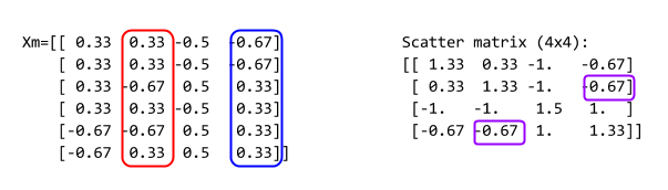
print 'Demeaned X:\n', rnd(Xm)
S = Xm.transpose()*Xm
G = Xm*Xm.transpose()
print 'Scatter matrix:\n', rnd(S)
print 'Gram Matrix:\n', rnd(G)

This produces the following output:


[[1 1 0 0]
 [1 1 0 0]
 [1 0 1 1]
 [1 1 0 1]
 [0 0 1 1]
 [0 1 1 1]]
Column means:  [[ 0.  0.  0.  0.]]
Column norms:  [ 1.15  1.15  1.22  1.15]
Demeaned X:
[[ 0.33  0.33 -0.5  -0.67]
 [ 0.33  0.33 -0.5  -0.67]
 [ 0.33 -0.67  0.5   0.33]
 [ 0.33  0.33 -0.5   0.33]
 [-0.67 -0.67  0.5   0.33]
 [-0.67  0.33  0.5   0.33]]
Scatter matrix:
[[ 1.33  0.33 -1.   -0.67]
 [ 0.33  1.33 -1.   -0.67]
 [-1.   -1.    1.5   1.  ]
 [-0.67 -0.67  1.    1.33]]
Gram Matrix:
[[ 0.92  0.92 -0.58  0.25 -0.92 -0.58]
 [ 0.92  0.92 -0.58  0.25 -0.92 -0.58]
 [-0.58 -0.58  0.92 -0.25  0.58 -0.08]
 [ 0.25  0.25 -0.25  0.58 -0.58 -0.25]
 [-0.92 -0.92  0.58 -0.58  1.25  0.58]
 [-0.58 -0.58 -0.08 -0.25  0.58  0.92]]

More on the Scatter Matrix

Because the scatter matrix is so important, I’m going to linger on it a bit.

Since the entries of the scatter matrix are dot products of column, we can think of them as dot products of the features that those columns represent. So the (2,3) entry compares the 2nd and 3rd feature. The dot product $a\cdot b = |a||b|\cos \theta$ , so the scatter matrix records a scaled version of the cosine similarity of the features. Cosine similarity measures the extent to which two vectors point in the same direction, opposite direction, or whether they’re simply orthogonal. Thus, the scatter matrix asks the extent to which two features ‘point’ in the same direction, multiplied by the overall scale of the features. Finally, since the dot product is commutative, the scatter matrix is symmetric.

If we were to add more data points, the scatter matrix would generally have a larger norm. It seems a bit silly to be so reactive to the size of the data set; if we rescale by the number of data points we get something a bit more robust. Indeed, if you multiply the scatter matrix by $\frac{1}{n-1}$ , you get the (sample) covariance matrix of X.

So the scatter matrix records vital statistical data about the relationship between features in our particular dataset.

Now, the singular value decomposition of $X$ is a product $U\Sigma V^t$ , where:

$U$ and $V^t$ are orthogonal matrices (so that $U^tU$ and $VV^t$ are identity matrices), and
$\Sigma$ is a diagonal matrix of the eigenvalues of $Xm$ (if $Xm$ is a square matrix).

But if we multiply the scatter matrix by $V$ , we get $SV = V\Sigma^2$ (try it!). This means that the columns of $V$ are eigenvectors for the scatter matrix. (Likewise, the column of $U^t$ are eigenvectors of the Gram matrix.)

We can express $X_m$ in terms of these eigenvectors by simply multiplying $XV = U\Sigma$ . This expression $U\Sigma$ is almost what we’re after.

Finally, PCA

The main idea of principal component analysis is to sort the eigenvalues $\Sigma$ and associated eigenvectors by size, and throw away the eigenvectors with small eigenvalues. The singular value decomposition $U\Sigma V^t$ usually consists of matrices of sizes $n\times p, p\times p$ , and $p\times p$ . Restricting to the $r$ largest eigenvalues reduces these sizes to $n\times r, r\times r$ , and $r\times p$ by throwing away (or zeroing out) rows and columns.

In this picture, we show the PCA obtained by keeping the two largest eigenvectors. Since the resulting data is two dimensional instead of four, we can plot it!

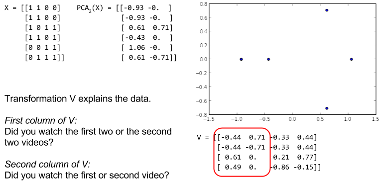
As indicated in the picture, when we squint at the columns of $V$ , we can make out what they’re saying about the data. The first is (roughly) asking whether someone tended to watch the first pair or second pair of movies. Looking at the matrix of data, this does seem like an important feature. And the second vector is asking whether someone watched the first or the second movie.

The beauty of PCA is that it makes asking these kinds of questions of the data automatic: What are the combinations of features (and in what amounts) that best decompose the data set?

Additionally, to apply PCA, we only have to keep the matrix $V$ and perform matrix multiplication on any new data points we encounter, assuming that the new data points are similar enough to our original training data.

Note that the sizes of the eigenvalues explicitly describe the contribution of each eigenvector to our dataset $X_m$ . As a result, removing the smallest eigenvectors has the least impact on the data. There’s another derivation of PCA in which one tries to find the best possible r-dimensional projection of the data $X_m$ , in terms of the error in ‘reconstructing’ data from its PCA representation. Minimizing this error leads directly to PCA decomposition with r components.

Further directions – Kernel PCA

The key takeaway here is that PCA comes down to understanding the relationship between features in your dataset, as measured by a dot product. However, there are many other ways to write down a relationship than just the dot product!

For example, we can make a new scatter matrix $S'$ whose entries are simply the cosines between the feature vectors, instead of the dot product. Or we could use an entirely different function, like: e^(-sum_k (Xik – Xjk)). (Sorry, I couldn’t get the latex to render in WordPress!). Suitably ‘good’ functions are called kernels. Doing an eigenvector analysis of the scatter matrix evaluated with a kernel function gives rise to kernel PCA. Kernel methods make it possible to find non-linear patterns in the data space.

You can find an implementation of kernel PCA in scikit-learn.

Further Directions – Respecting Data Segmentation

If your data naturally clusters into major segments with radically different behaviour, the standard PCA may not do a great job of describing your data. Instead, you can perform some segmentation or pre-clustering, and then apply a different PCA decomposition to each of the different data clusters.

Further Directions – Probabilistic PCA

Bishop’s Machine Learning and Pattern Recognition book describes a couple nice probability-based interpretations of PCA. The first allows computation of the PCA iteratively using an EM algorithm, which can be faster than explicitly computing eigenvectors with certain large datasets. Bishop also describes a Bayesian approach to determine the number of components one should actually keep.

Inventing Situations.

tom denton on math and things.